Principal component analysis (PCA) is a dimensionality reduction technique for machine learning. PCA projects the data into lower-dimensional space; it does not change the data and therefore all of the information of the dataset is preserved (although PCA does come at a cost of some accuracy). PCA can be used to aid in data visualization, to increase the efficiency of algorithms (by reducing the number of dimensions and removing noise, redundancy and multicollinearity in the data), and for feature extraction. Principal components are new, uncorrelated variables that are linear combinations of the original variables. The first component will be the projection that describes the most variance in the data. The second will be orthogonal to the first and capture the most most remaining variance, and so on. An $n$-dimensional dataset will have $n$ principal components, but with PCA we select the top $p$ components for further analysis. 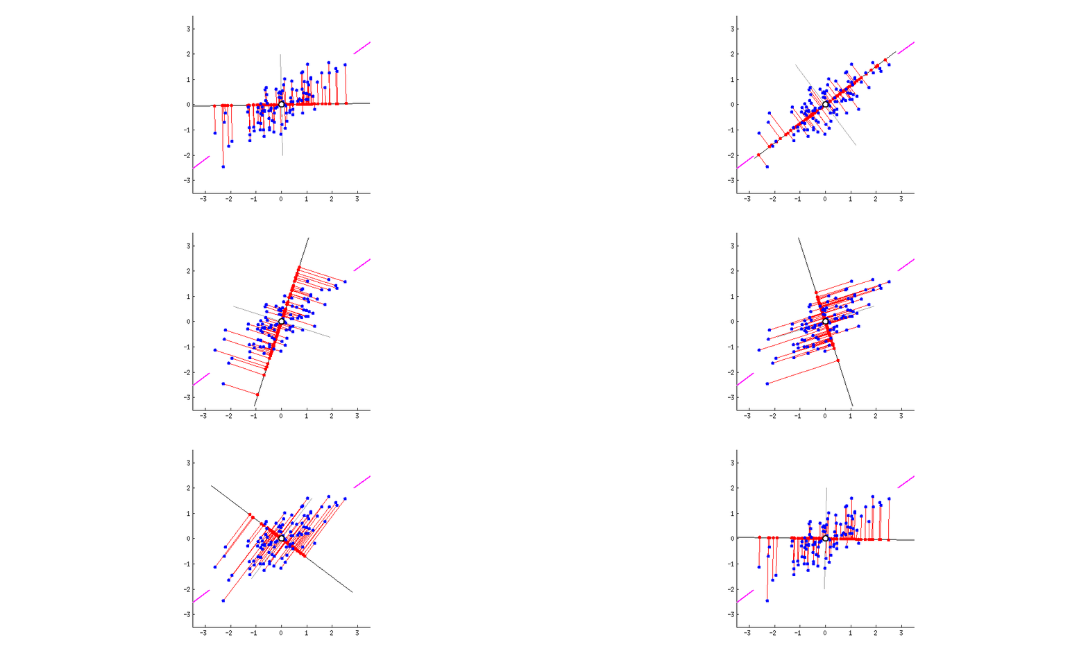This chart from [Principal Component Analysis (PCA): A step-by-step explanation](https://builtin.com/data-science/step-step-explanation-principal-component-analysis) helps visualize how the principal components are selected. Geometrically, the component will be the line that maximizes the variance (indicated by the purple end lines).  The number of principle components to use must be selected by the analyst, one way is to look for an "elbow" in a graph of the explained variance against the number of components, another is to set a hard threshold, selecting the number of components that explain $x\%$ of the variability. The process for PCA is 1. [[Standardize]] the range of continuous initial variables. PCA is sensitive to variable scaling. 2. Compute the [[covariance matrix]] to identify correlations 3. Compute the eigenvectors and eigenvalues of the covariance matrix to identify the principal components 4. Create a feature vector to decide which principal components to keep 5. Recast the data along the principal components axes PCA is an eigen decomposition of the covariance matrix $X^T X$. The eigenvectors of the covariance matrix are the directions of the axes where there is the most variance, the principal components. The corresponding eigenvalues give the amount of variance carried in each principle component. Ranking the eigenvectors in order of their eigenvalues, highest to lowest, returns the principal components in order of significance. To compute the percentage of variance (information) accounted for by each component, divide the eigenvalue of each component by the sum of eigenvalues. The feature vector is the matrix that includes as columns the eigenvectors of the top $p$ principal components. It can be possible to interpret these components by writing out their form and using domain knowledge to understand their implications. See [Visually Explained - Principal Component Analysis (PCA) - YouTube](https://youtu.be/FD4DeN81ODY?si=QXTGAUZKKai0kvBD) for a great example. Another approach to PCA is singular value decomposition (SVD). SVD is more efficient than PCA. The [[Python]] package `sklearn` uses singular value decomposition under the hood for calculating the principal components. ```python sklearn.decomposition.PCA pca = PCA(n_components=2).fit(X) x_reduced = PCA(n_components=2).fit_transform(X) pca.components_ pca.explained_variance_ratio ``` > [!Tip]- Additional Resources > - [Principal Component Analysis (PCA): A step-by-step explanation](https://builtin.com/data-science/step-step-explanation-principal-component-analysis) > - [Visually Explained - Principal Component Analysis (PCA) - YouTube](https://youtu.be/FD4DeN81ODY?si=QXTGAUZKKai0kvBD)